scFeatureFilter:

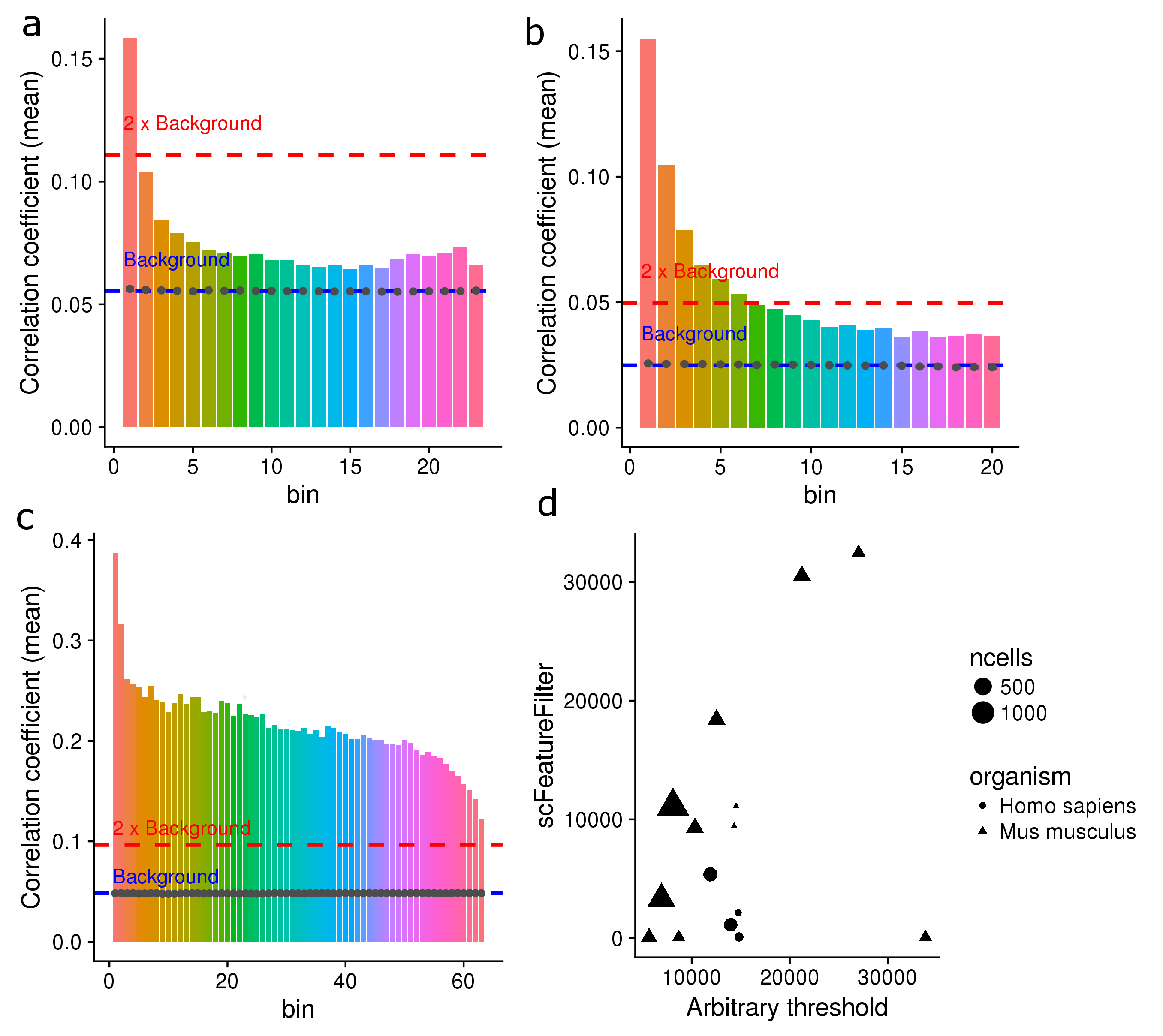
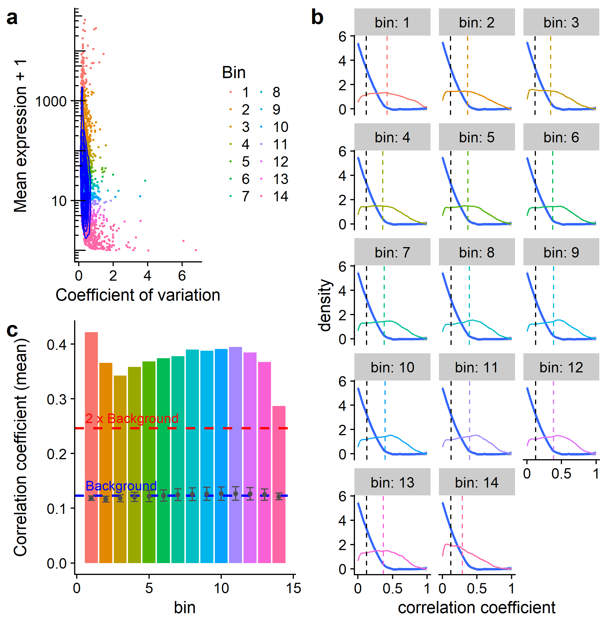
# scFeatureFilter:
## correlation-based feature filtering for single-cell RNA-seq
### <span class="citation">@G_Devailly</span>
### 2018/01/17

---

# Introduction

- Single cell RNA-sequencing is increasingly popular.

- scRNA-seq is noisier than bulk RNA-seq.

- Filtering of noisy, lowly-expressed features.red[*] is common.

---

## Introduction
- Using spike-in RNA information

- Arbitrary filtering:

>.small[[...] on a filtered data set, where we retain only genes with an estimated
TPM above 1 in more than 25% of the considered cells. (1)]
 
>.small[Genes with less than 5 reads and expressed in
less than 10 cells were removed. (2)] 
 
>.small[Here, low-abundance genes are defined as those 
with an average count below a filter threshold of 1 [count]. (3)] 
 
>.small[ Genes were filtered, keeping 15,633 out of 26,178 genes
that were expressed in at least 5 out of 1,919 sequenced cells (RPKM 
≥ 10) and for which cells with expression came from at least 
two different embryos. (4)]

.tiny[.red[1] Soneson & Robinson, bioRxiv, 2017  
.red[2] Stevant et al., bioRxiv, 2017  
.red[3] Lun et al., F1000Research, 2016  
.red[4] Petropulos et al., Cell, 2016]

---

## Introduction

- No standard threshold for filtering.

- Same threshold might not be of the *same stringency*
in different datasets, notably across species.red[*].

* Can we do better?

---

- Available on GitHub:  
[github.com/gdevailly/scFeatureFilte](https://github.com/gdevailly/scFeatureFilter)

- Accepted in [Bioconductor](https://www.bioconductor.org/packages/devel/bioc/html/scFeatureFilter.html)

- Might help to set a relevant expression threshold for feature filtering.

```r
library(scFeatureFilter)
```

---

## Example datasets:
32 scRNA-seq of human embryonic stem cells .small[(Yan et al., Nat Struct Mol Biol, 2013.)]

```r
dim(scData_hESC)
## [1] 60468    33
```

```r
scData_hESC
```

.small[
|gene               | cell_1| cell_2| cell_3| cell_4|
|:------------------|------:|------:|------:|------:|
|ENSG00000000003.13 |  55.33|  35.98|  53.68|  31.95|
|ENSG00000000005.5  |   0.00|   0.00|   0.13|   0.00|
|ENSG00000000419.11 |  53.97|  55.47|  41.87| 110.75|
|ENSG00000000457.12 |   0.92|   0.22|   0.65|   0.87|
]

.small[Expression matrices can  be either `data.frame`, `tibble`, `matrix` or `SingleCellExperiment`.]

---

## Mean-variance exploration:

```r
calculate_cvs(scData_hESC, max_zeros = 0.75)[1:4, 1:5]
## # A tibble: 4 x 5
##             geneName      mean        sd        cv
##                <chr>     <dbl>     <dbl>     <dbl>
## 1 ENSG00000000003.13 70.022328 73.332127 1.0472678
## 2  ENSG00000000005.5  1.000291  2.527535 2.5267987
## 3 ENSG00000000419.11 80.991847 71.534922 0.8832361
## 4 ENSG00000000457.12  1.590995  1.804686 1.1343132
## # ... with 1 more variables: GSM922224_hESCpassage0_Cell4_0 <dbl>
```
`max_zeros`: maximum proportion of `0` value for a feature to be kept

---

## Mean-variance exploration:

```r
calculate_cvs(scData_hESC, max_zeros = 0.75) %>%
    plot_mean_variance(colourByBin = FALSE) +
    annotation_logticks(sides = "l")
```

---

## Binning of the genes:

```r
scData_hESC %>%
    calculate_cvs %>%
    define_top_genes(window_size = 100) %>%
    bin_scdata(window_size = 1000) %>%
    plot_mean_variance() +
    annotation_logticks(sides = "l")
```

---
## Assumptions

.pull-left[
<img src="devailly_scFeatureFilter_files/figure-html/meanVar3-1.png" width="100%" style="display: block; margin: auto;" />
]
.pull-right[
- high expression = less technical variation

- biological variation = transcription module

- correlation of genes belonging to the same transcription module
]

---

## Correlation of the data:
- **A reference set of genes**: the top bin

- Three control sets of genes: shuffling of the expression values of the reference set

Each gene in each bin is correlated against each gene in the **reference set**, and each gene in the 3 **control sets**:

```r
corDistrib <- scData_hESC %>%
    calculate_cvs %>%
    define_top_genes(window_size = 100) %>%
    bin_scdata(window_size = 1000) %>%
    correlate_windows(n_random = 3)
## Mean expression of last top gene: 2114.40221875
## Number of windows: 18
```

---

## Correlation of the data

```r
corDens <- correlations_to_densities(corDistrib)
plot_correlations_distributions(corDens, facet_ncol = 6) +
    scale_x_continuous(breaks = c(0, 0.5, 1), labels = c("0", "0.5", "1"))
```

---

## Correlation of the data

```r
metrics <- get_mean_median(corDistrib)
plot_correlations_distributions(corDens,  metrics = metrics, facet_ncol = 6) +
    scale_x_continuous(breaks = c(0, 0.5, 1), labels = c("0", "0.5", "1"))
```

---

## Threshold decision

```r
plot_metric(metrics, show_ctrl = FALSE, show_threshold = FALSE)
```

---

## Threshold decision

```r
plot_metric(metrics, show_ctrl = TRUE, show_threshold = FALSE)
```

---

## Threshold decision

```r
plot_metric(metrics, show_ctrl = TRUE, show_threshold = TRUE, threshold = 2)
```

---

## Geting back the filtered expression matrix:

```r
binned_data <- scData_hESC %>%
    calculate_cvs %>%
    define_top_genes(window_size = 100) %>%
    bin_scdata(window_size = 1000)
```

```r
determine_bin_cutoff(metrics, threshold = 2)
## [1] 9

filtered_data <- filter_expression_table(
    binned_data,
    bin_cutoff = determine_bin_cutoff(metrics)
)

nrow(scData_hESC)
## [1] 60468

nrow(binned_data)
## [1] 17929

nrow(filtered_data)
## [1] 7442
```

---
# A shortcut:

```r
filtered_data <- sc_feature_filter(scData_hESC)
## Mean expression of last top gene: 2114.40221875
## Number of windows: 18

dim(scData_hESC)
## [1] 60468    33

dim(filtered_data)
## [1] 7442   33
```

---

---
class: center

## Testing `scFeatureFilter` on more datasets:  
.medium[16 datasets from [ConquerDB](http://imlspenticton.uzh.ch:3838/conquer/) (human and mouse)]
![:scale 68%](img/conquer.png)

---
class: center

## `scFeatureFilter` on bulk RNA-seq:  
.medium[48 repplicated bulk RNA-seq (yeast)] .tiny[(Gierlinski et al., Bioinformatics, 2015)]
![:scale 60%](img/yeast.png)

---
class: inverse

# Limits of `scFeatureFilter`

---
## Lots of parameters?
.medium[
|parameter           |description                                       |default|
|:-------------------|:-------------------------------------------------|------:|
|`max_zeros`         | maximum proportion of 0 for a feature to be kept |   0.75|
|`top_window_size`   | size of the reference set                        |    100|
|`other_window_size` | size of the other bins                           |   1000|
|`threshold`         | stringency of the selection                      |      2|
]

---

## Lots of parameters?
The method is robust to `other_window_size`:

---
## Robust to `max_zeros`?
high proportion of 0s ~= low expression

- mostly not in the reference set

- more abundant in the low expression bins

- less abundant in the high expression bins

## `threshold` is a feature
`threshold`: More or less stringency depending of the use cases and user preference.

---

## `top_window_size`
`top_window_size` can have *massive* impact:

- if **too big**: Risk of selecting everything.
- if **too small**: Might not capture enough biological variation.

~100 seems to be a sweet spot on mouse and human data.

---
## `top_window_size`
Average auto-correlation of the top window depending on its size:

```r
plot_top_window_autocor(calculate_cvs(scData_hESC))
```

---

# Other limits?

- Tested on a dataset with 1378 cells. Scalable until when?

- Not designed nor tested for 10x genomics scRNA-seq.

---
class: inverse

# Conclusion:
`scFeatureFilter`: an R package for less arbitrary threshold selection

We are looking for feedback:
- Usefull?

- Overkilled?

- Broken assumptions?

- Better existing methods?

---

Anagha Joshi

Angeles Arzalluz-Luque

Anna Mantsoki
]
.pull-right[
![:scale 78%](img/logo.png)
]